factors_r <- c("SP500", "DTWEXAFEGS") # "SP500" does not contain dividends; note: "DTWEXM" discontinued as of Jan 2020
factors_d <- c("DGS10", "BAMLH0A0HYM2")

Black-Scholes model

level_shock <- function(shock, S, tau, sigma) {
  
  result <- S * (1 + shock * sigma * sqrt(tau))
  
  return(result)
  
}

factor <- "SP500"
types <- c("call", "put")
S <- as.numeric(zoo::coredata(zoo::na.locf(levels_xts[nrow(levels_xts), factor]))) # Recycling array of length 1 in vector-array arithmetic is deprecated. Use c() or as.vector() instead.
K <- S
r <- 0 # use "USD3MTD156N"
q <- 0 # see https://stackoverflow.com/a/11286679 
tau <- 1 # = 252 / 252
sigma <- as.numeric(zoo::coredata(sd_xts[nrow(sd_xts), factor])) # use "VIXCLS"
shocks <- seq(-3, 3, by = 0.5)

greeks_dt <- data.table::CJ(type = types, shock = shocks)
greeks_dt[ , spot := level_shock(shock, S, tau, sigma), by = c("type", "shock")]

Value

For a given spot price \(S\), strike price \(K\), risk-free rate \(r\), annual dividend yield \(q\), time-to-maturity \(\tau = T - t\), and volatility \(\sigma\):

\[ \begin{aligned} V_{c}&=Se^{-q\tau}\Phi(d_{1})-e^{-r\tau}K\Phi(d_{2}) \\ V_{p}&=e^{-r\tau}K\Phi(-d_{2})-Se^{-q\tau}\Phi(-d_{1}) \end{aligned} \]

bs_value <- function(type, S, K, r, q, tau, sigma, d1, d2) {

  r_df <- exp(-r * tau)
  q_df <- exp(-q * tau)
  
  call_value <- S * q_df * Phi(d1) - r_df * K * Phi(d2)
  put_value <- r_df * K * Phi(-d2) - S * q_df * Phi(-d1)
  result <- ifelse(type == "call", call_value, put_value)
  
  return(result)
  
}

where

\[ \begin{aligned} d_{1}&={\frac{\ln(S/K)+(r-q+\sigma^{2}/2)\tau}{\sigma{\sqrt{\tau}}}} \\ d_{2}&={\frac{\ln(S/K)+(r-q-\sigma^{2}/2)\tau}{\sigma{\sqrt{\tau}}}}=d_{1}-\sigma{\sqrt{\tau}} \\ \phi(x)&={\frac{e^{-{\frac {x^{2}}{2}}}}{\sqrt{2\pi}}} \\ \Phi(x)&={\frac{1}{\sqrt{2\pi}}}\int_{-\infty}^{x}e^{-{\frac{y^{2}}{2}}}dy=1-{\frac{1}{\sqrt{2\pi}}}\int_{x}^{\infty}e^{-{\frac{y^{2}}{2}}dy} \end{aligned} \]

bs_d1 <- function(S, K, r, q, tau, sigma) {
  
  result <- (log(S / K) + (r - q + sigma ^ 2 / 2) * tau) / (sigma * sqrt(tau))
  
  return(result)
  
}

bs_d2 <- function(S, K, r, q, tau, sigma) {
  
  result <- (log(S / K) + (r - q - sigma ^ 2 / 2) * tau) / (sigma * sqrt(tau))
  
  return(result)
  
}

phi <- function(x) {
  
  result <- dnorm(x)
  
  return(result)
  
}

Phi <- function(x) {
  
  result <- pnorm(x)
  
  return(result)
  
}

greeks_dt[ , d1 := bs_d1(spot, K, r, q, tau, sigma), by = c("type", "shock")]
greeks_dt[ , d2 := bs_d2(spot, K, r, q, tau, sigma), by = c("type", "shock")]
greeks_dt[ , value := bs_value(type, spot, K, r, q, tau, sigma, d1, d2), by = c("type", "shock")]

First-order

Delta

\[ \begin{aligned} \Delta_{c}&={\frac{\partial V_{c}}{\partial S}}=e^{-q\tau}\Phi(d_{1}) \\ \Delta_{p}&={\frac{\partial V_{p}}{\partial S}}=-e^{-q\tau}\Phi(-d_{1}) \end{aligned} \]

bs_delta <- function(type, S, K, r, q, tau, sigma, d1, d2) {
  
  q_df <- exp(-q * tau)

  call_value <- q_df * Phi(d1)
  put_value <- -q_df * Phi(-d1)
  result <- ifelse(type == "call", call_value, put_value)
  
  return(result)
  
}

greeks_dt[ , delta := bs_delta(type, spot, K, r, q, tau, sigma, d1, d2), by = c("type", "shock")]

Delta-beta

Notional market value is the market value of a leveraged position:

\[ \begin{aligned} \text{Equity options }=&\,\#\text{ contracts}\times\text{multiple}\times\text{spot price}\\ \text{Delta-adjusted }=&\,\#\text{ contracts}\times\text{multiple}\times\text{spot price}\times\text{delta} \end{aligned} \]

https://en.wikipedia.org/wiki/Notional_amount

bs_delta_diff <- function(type, S, K, r, q, tau, sigma, delta0) {
  
  d1 <- bs_d1(S, K, r, q, tau, sigma)
  d2 <- bs_d2(S, K, r, q, tau, sigma)
  delta <- bs_delta(type, S, K, r, q, tau, sigma, d1, d2)
  
  call_value <- delta - delta0
  put_value <- delta0 - delta
  
  result <- ifelse(type == "call", call_value, put_value)
      
  return(result)
  
}

beta <- 0.35
type <- "call"
n <- 1
multiple <- 100
total <- 1000000

d1 <- bs_d1(S, K, r, q, tau, sigma)
d2 <- bs_d2(S, K, r, q, tau, sigma)
sec <- list(
  "n" = n,
  "multiple" = multiple,
  "S" = S,
  "delta" = bs_delta(type, S, K, r, q, tau, sigma, d1, d2),
  "beta" = 1
)

beta_dt <- data.table::CJ(type = type, shock = shocks)
beta_dt[ , spot := level_shock(shock, S, tau, sigma), by = c("type", "shock")]
beta_dt[ , static := beta]
beta_dt[ , diff := bs_delta_diff(type, spot, K, r, q, tau, sigma, sec[["delta"]])]
beta_dt[ , dynamic := beta + sec[["n"]] * sec[["multiple"]] * sec[["S"]] * sec[["beta"]] * diff / total, by = c("type", "shock")]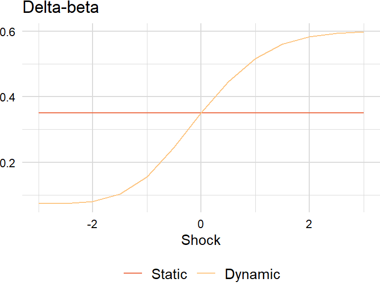

For completeness, duration equivalent is defined as:

\[ \begin{aligned} \text{10-year equivalent }=\,&\frac{\text{security duration}}{\text{10-year OTR duration}} \end{aligned} \]

Vega

\[ \begin{aligned} \nu_{c,p}&={\frac{\partial V_{c,p}}{\partial\sigma}}=Se^{-q\tau}\phi(d_{1}){\sqrt{\tau}}=Ke^{-r\tau}\phi(d_{2}){\sqrt{\tau}} \end{aligned} \]

bs_vega <- function(type, S, K, r, q, tau, sigma, d1, d2) {
  
  q_df <- exp(-q * tau)
  
  result <- S * q_df * phi(d1) * sqrt(tau)
  
  return(result)
  
}

greeks_dt[ , vega := bs_vega(type, spot, K, r, q, tau, sigma, d1, d2), by = c("type", "shock")]

Theta

\[ \begin{aligned} \Theta_{c}&=-{\frac{\partial V_{c}}{\partial \tau}}=-e^{-q\tau}{\frac{S\phi(d_{1})\sigma}{2{\sqrt{\tau}}}}-rKe^{-r\tau}\Phi(d_{2})+qSe^{-q\tau}\Phi(d_{1}) \\ \Theta_{p}&=-{\frac{\partial V_{p}}{\partial \tau}}=-e^{-q\tau}{\frac{S\phi(d_{1})\sigma}{2{\sqrt{\tau}}}}+rKe^{-r\tau}\Phi(-d_{2})-qSe^{-q\tau}\Phi(-d_{1}) \end{aligned} \]

bs_theta <- function(type, S, K, r, q, tau, sigma, d1, d2) {
  
  r_df <- exp(r * tau)
  q_df <- exp(q * tau)

  call_value <- -q_df * S * phi(d1) * sigma / (2 * sqrt(tau)) -
    r * K * r_df * Phi(d2) + q * S * q_df * Phi(d1)
  
  put_value <- -q_df * S * phi(d1) * sigma / (2 * sqrt(tau)) +
    r * K * r_df * Phi(-d2) - q * S * q_df * Phi(-d1)
      
  result <- ifelse(type == "call", call_value, put_value)
  
  return(result)
  
}

greeks_dt[ , theta := bs_theta(type, spot, K, r, q, tau, sigma, d1, d2), by = c("type", "shock")]

Second-order

Gamma

\[ \begin{aligned} \Gamma_{c,p}&={\frac{\partial\Delta_{c,p}}{\partial S}}={\frac{\partial^{2}V_{c,p}}{\partial S^{2}}}=e^{-q\tau}{\frac{\phi(d_{1})}{S\sigma{\sqrt{\tau}}}}=Ke^{-r\tau}{\frac{\phi(d_{2})}{S^{2}\sigma{\sqrt{\tau}}}} \end{aligned} \]

bs_gamma <- function(type, S, K, r, q, tau, sigma, d1, d2) {

  q_df <- exp(-q * tau)
  
  result <- q_df * phi(d1) / (S * sigma * sqrt(tau))
  
  return(result)
  
}

greeks_dt[ , gamma := bs_gamma(type, spot, K, r, q, tau, sigma, d1, d2), by = c("type", "shock")]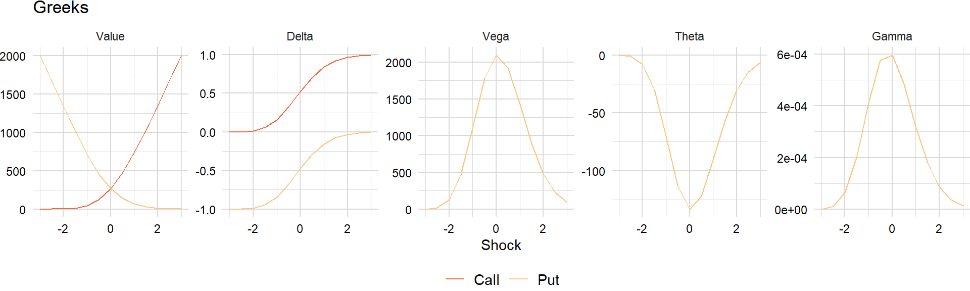

Taylor series

First-order

Price-yield formula

For a function of one variable, \(f(x)\), the Taylor series formula is:

\[ \begin{aligned} f(x+\Delta x)&=f(x)+{\frac{f'(x)}{1!}}\Delta x+{\frac{f''(x)}{2!}}(\Delta x)^{2}+{\frac{f^{(3)}(x)}{3!}}(\Delta x)^{3}+\cdots+{\frac{f^{(n)}(x)}{n!}}(\Delta x)^{n}+\cdots\\ f(x+\Delta x)-f(x)&={\frac{f'(x)}{1!}}\Delta x+{\frac{f''(x)}{2!}}(\Delta x)^{2}+{\frac{f^{(3)}(x)}{3!}}(\Delta x)^{3}+\cdots+{\frac{f^{(n)}(x)}{n!}}(\Delta x)^{n}+\cdots \end{aligned} \]

Using the price-yield formula, the estimated percentage change in price for a change in yield is:

\[ \begin{aligned} P(y+\Delta y)-P(y)&\approx{\frac{P'(y)}{1!}}\Delta y+{\frac{P''(y)}{2!}}(\Delta y)^{2}\\ &\approx -D\Delta y +{\frac{C}{2!}}(\Delta y)^{2} \end{aligned} \]

pnl_bond <- function(duration, convexity, dy) {
  
  duration_pnl <- -duration * dy
  convexity_pnl <- (convexity / 2) * dy ^ 2
  income_pnl <- dy
  
  result <- list(
    "total" = duration_pnl + convexity_pnl + income_pnl,
    "duration" = duration_pnl,
    "convexity" = convexity_pnl,
    "income" = income_pnl
  )
  
  return(result)
  
}

factor <- "DGS10"
duration <- 6.5
convexity <- 0.65
y <- zoo::coredata(tail(zoo::na.locf(levels_xts[ , factor]), width)[1])

bonds_dt <- data.table::data.table(index = zoo::index(tail(levels_xts, width)),
                                   duration = duration, convexity = convexity,
                                   dy = zoo::na.locf(tail(levels_xts[ , factor], width)))
data.table::setnames(bonds_dt, c("index", "duration", "convexity", "dy"))
bonds_dt[ , dy := (dy - y) / 100, by = index]

attrib_dt <- bonds_dt[ , as.list(unlist(pnl_bond(duration, convexity, dy))), by = index]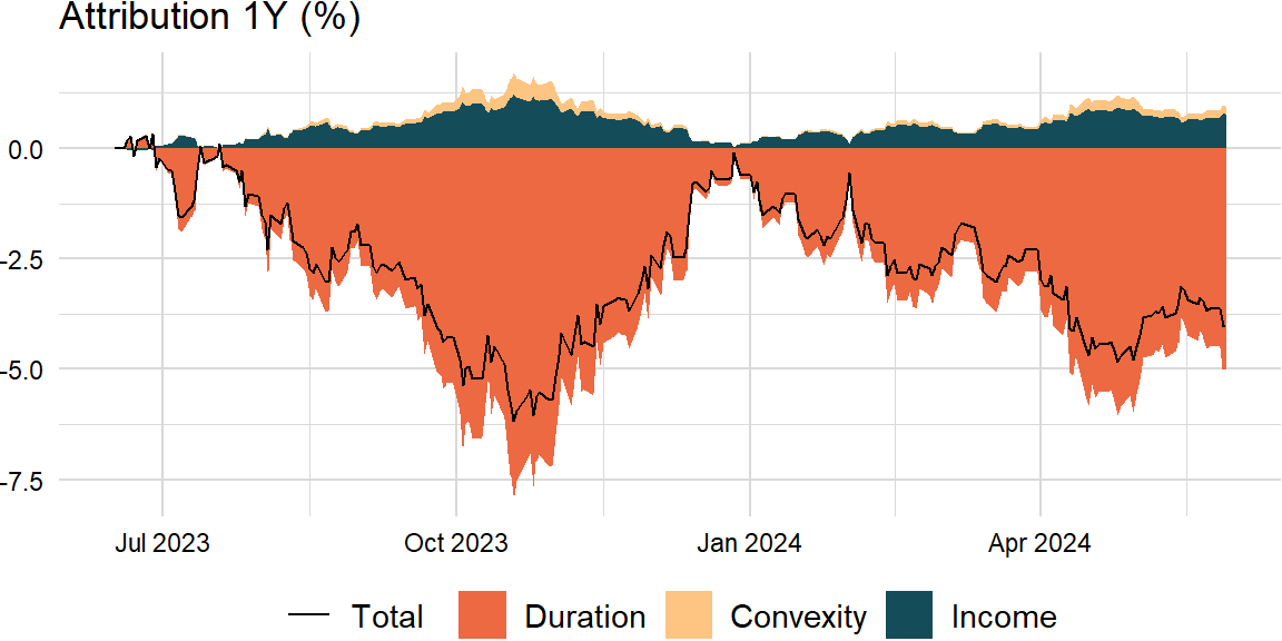

Duration-yield formula

The derivative of duration with respect to interest rates gives:

\[ \begin{aligned} \text{Drift}&=\frac{\partial D}{\partial y}=\frac{\partial}{\partial y}\left(-\frac{1}{P}\frac{\partial D}{\partial y}\right)\\ &=-\frac{1}{P}\frac{\partial^{2}P}{\partial y^{2}}+\frac{1}{P^{2}}\frac{\partial P}{\partial y}\frac{\partial P}{\partial y}\\ &=-C+D^{2} \end{aligned} \]

Because of market conventions, use the following formula: \(\text{Drift}=\frac{1}{100}\left(-C\times 100+D^{2}\right)=-C+\frac{D^{2}}{100}\). For example, if convexity and yield are percent then \(\text{Drift}=\left(-0.65+\frac{6.5^{2}}{100}\right)\partial y\times100\) or basis points then \(\text{Drift}=\left(-65+6.5^{2}\right)\partial y\).

yield_shock <- function(shock, tau, sigma) {
  
  result <- shock * sigma * sqrt(tau)
  
  return(result)
  
}

duration_drift <- function(duration, convexity, dy) {
  
  drift <- -convexity + duration ^ 2 / 100
  change <- drift * dy * 100
  
  result <- list(
    "drift" = drift,
    "change" = change
  )
  
  return(result)
  
}

# "Risk Management: Approaches for Fixed Income Markets" (page 45)
factor <- "DGS10"
sigma <- zoo::coredata(sd_xts[nrow(sd_xts), factor])

duration_dt <- data.table::CJ(shock = shocks)
duration_dt[ , spot := yield_shock(shock, tau, sigma), by = "shock"]
duration_dt[ , static := duration]
duration_dt[ , dynamic := duration + duration_drift(duration, convexity, spot)[["change"]], by = "shock"]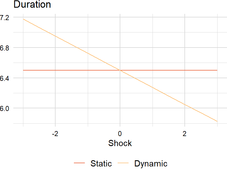

Second-order

Black’s formula

A similar formula holds for functions of several variables \(f(x_{1},\ldots,x_{n})\). This is usually written as:

\[ \begin{aligned} f(x_{1}+\Delta x_{1},\ldots,x_{n}+\Delta x_{n})&=f(x_{1},\ldots, x_{n})+ \sum _{j=1}^{n}{\frac{\partial f(x_{1},\ldots,x_{n})}{\partial x_{j}}}(\Delta x_{j})\\ &+{\frac {1}{2!}}\sum_{j=1}^{n}\sum_{k=1}^{n}{\frac{\partial^{2}f(x_{1},\ldots,x_{d})}{\partial x_{j}\partial x_{k}}}(\Delta x_{j})(\Delta x_{k})+\cdots \end{aligned} \]

Using Black’s formula, the estimated change of an option price is:

\[ \begin{aligned} V(S+\Delta S,\sigma+\Delta\sigma,t+\Delta t)-V(S,\sigma,t)&\approx{\frac{\partial V}{\partial S}}\Delta S+{\frac{1}{2!}}{\frac{\partial^{2}V}{\partial S^{2}}}(\Delta S)^{2}+{\frac{\partial V}{\partial \sigma}}\Delta\sigma+{\frac{\partial V}{\partial t}}\Delta t\\ &\approx \Delta_{c,p}\Delta S+{\frac{1}{2!}}\Gamma_{c,p}(\Delta S)^{2}+\nu_{c,p}\Delta\sigma+\Theta_{c,p}\Delta t \end{aligned} \]

https://quant-next.com/option-greeks-and-pl-decomposition-part-1/

pnl_option <- function(type, S, K, r, q, tau, sigma, dS, dt, dsigma) {
  
  d1 <- bs_d1(S, K, r, q, tau, sigma)
  d2 <- bs_d2(S, K, r, q, tau, sigma)
  value <- bs_value(type, S, K, r, q, tau, sigma, d1, d2)
  delta <- bs_delta(type, S, K, r, q, tau, sigma, d1, d2)
  vega <- bs_vega(type, S, K, r, q, tau, sigma, d1, d2)
  theta <- bs_theta(type, S, K, r, q, tau, sigma, d1, d2)
  gamma <- bs_gamma(type, S, K, r, q, tau, sigma, d1, d2)
  
  delta_pnl <- delta * dS / value
  gamma_pnl <- gamma / 2 * dS ^ 2 / value
  vega_pnl <- vega * dsigma / value
  theta_pnl <- theta * dt / value
  
  result <- list(
    "total" = delta_pnl + gamma_pnl + vega_pnl + theta_pnl,
    "delta" = delta_pnl,
    "gamma" = gamma_pnl,
    "vega" = vega_pnl,
    "theta" = theta_pnl
  )
  
  return(result)    
  
}

factor <- "SP500"
type <- "call"
S <- zoo::coredata(tail(zoo::na.locf(levels_xts[ , factor]), width)[1])
K <- S # * (1 + 0.05)
tau <- 1 # = 252 / 252
sigma <- zoo::coredata(tail(sd_xts[ , factor], width)[1])

options_dt <- data.table::data.table(index = zoo::index(tail(levels_xts, width)),
                                     spot = zoo::na.locf(tail(levels_xts[ , factor], width)),
                                     sigma = tail(sd_xts[ , factor], width))
data.table::setnames(options_dt, c("index", "spot", "sigma"))
options_dt[ , dS := spot - S, by = index]
options_dt[ , dt_diff := as.numeric(index - index[1])]
options_dt[ , dt := dt_diff / tail(dt_diff, 1)]
options_dt[ , dsigma := sigma - ..sigma, by = index]

attrib_dt <- options_dt[ , as.list(unlist(pnl_option(type, S, K, r, q, tau, ..sigma,
                                                     dS, dt, dsigma))), by = index]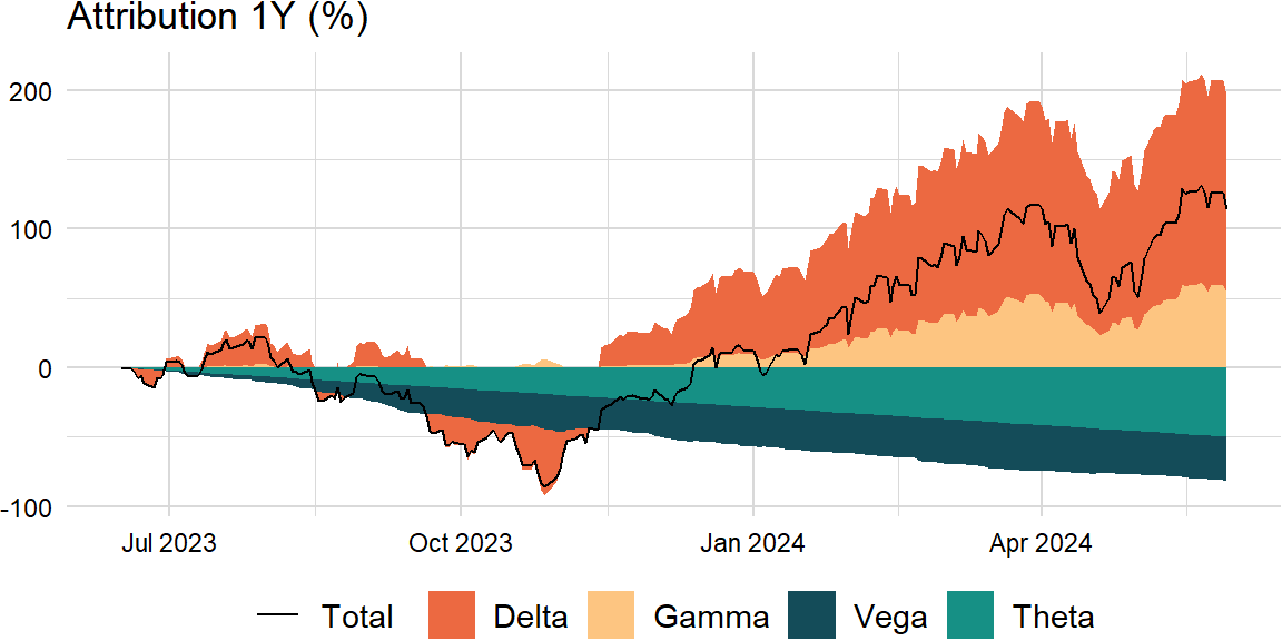

Ito’s lemma

For a given diffiusion \(X(t, w)\) driven by:

\[ \begin{aligned} dX_{t}&=\mu_{t}dt+\sigma_{t}dB_{t} \end{aligned} \]

Then proceed with the Taylor series for a function of two variables \(f(t,x)\):

\[ \begin{aligned} df&={\frac{\partial f}{\partial t}}dt+{\frac{\partial f}{\partial x}}dx+{\frac{1}{2}}{\frac{\partial^{2}f}{\partial x^{2}}}dx^{2}\\ &={\frac{\partial f}{\partial t}}dt+{\frac{\partial f}{\partial x}}(\mu_{t}dt+\sigma_{t}dB_{t})+{\frac{1}{2}}{\frac{\partial^{2}f}{\partial x^{2}}}\left(\mu_{t}^{2}dt^{2}+2\mu_{t}\sigma _{t}dtdB_{t}+\sigma_{t}^{2}dB_{t}^{2}\right)\\ &=\left({\frac{\partial f}{\partial t}}+\mu_{t}{\frac{\partial f}{\partial x}}+{\frac{\sigma _{t}^{2}}{2}}{\frac{\partial ^{2}f}{\partial x^{2}}}\right)dt+\sigma_{t}{\frac{\partial f}{\partial x}}dB_{t} \end{aligned} \]

Note: set the \(dt^{2}\) and \(dtdB_{t}\) terms to zero and substitute \(dt\) for \(dB^{2}\).

Geometric Brownian motion

The most common application of Ito’s lemma in finance is to start with the percent change of an asset:

\[ \begin{aligned} \frac{dS}{S}&=\mu_{t}dt+\sigma_{t}dB_{t} \end{aligned} \]

Then apply Ito’s lemma with \(f(S)=log(S)\):

\[ \begin{aligned} d\log(S)&=f^{\prime}(S)dS+{\frac{1}{2}}f^{\prime\prime}(S)S^{2}\sigma^{2}dt\\ &={\frac {1}{S}}\left(\sigma SdB+\mu Sdt\right)-{\frac{1}{2}}\sigma^{2}dt\\ &=\sigma dB+\left(\mu-{\tfrac{\sigma^{2}}{2}}\right)dt \end{aligned} \]

It follows that:

\[ \begin{aligned} \log(S_{t})-\log(S_{0})=\sigma dB+\left(\mu-{\tfrac{\sigma^{2}}{2}}\right)dt \end{aligned} \]

Exponentiating gives the expression for \(S\):

\[ \begin{aligned} S_{t}=S_{0}\exp\left(\sigma B_{t}+\left(\mu-{\tfrac{\sigma^{2}}{2}}\right)t\right) \end{aligned} \]

This provides a recursive procedure for simulating values of \(S\) at \(t_{0}<t_{1}<\cdots<t_{n}\):

\[ \begin{aligned} S(t_{i+1})&=S(t_{i})\exp\left(\sigma\sqrt{t_{i+1}-t_{i}}Z_{i+1}+\left[\mu-{\tfrac{\sigma^{2}}{2}}\right]\left(t_{i+1}-t_{i}\right)\right) \end{aligned} \]

where \(Z_{1},Z_{2},\ldots,Z_{n}\) are independent standard normals.

sim_gbm <- function(n_sim, S, mu, sigma, dt) {
  
  result <- S * exp(cumsum(sigma * sqrt(dt) * rnorm(n_sim)) +
                    (mu - 0.5 * sigma ^ 2) * dt)
  
  return(result)
  
}

This leads to an algorithm for simulating a multidimensional geometric Brownian motion:

\[ \begin{aligned} S_{k}(t_{i+1})&=S_{k}(t_{i})\exp\left(\sqrt{t_{i+1}-t_{i}}\sum_{j=1}^{d}{A_{kj}Z_{i+1,j}}+\left[\mu_{k}-{\tfrac{\sigma_{k}^{2}}{2}}\right]\left(t_{i+1}-t_{i}\right)\right) \end{aligned} \]

where \(A\) is the Cholesky factor of \(\Sigma\), i.e. \(A\) is any matrix for which \(AA^\mathrm{T}=\Sigma\).

sim_multi_gbm <- function(n_sim, S, mu, sigma, dt) {
  
  n_cols <- ncol(sigma)
  
  Z <- matrix(rnorm(n_sim * n_cols), nrow = n_sim, ncol = n_cols)
  X <- sweep(sqrt(dt) * (Z %*% chol(sigma)), 2, (mu - 0.5 * diag(sigma)) * dt, "+")
  
  result <- sweep(apply(X, 2, function(x) exp(cumsum(x))), 2, S, "*")
  
  return(result)
  
}

S <- rep(1, length(factors))
sigma <- cov(returns_xts, use = "complete.obs") * scale[["periods"]]
mu <- colMeans(na.omit(returns_xts)) * scale[["periods"]]
mu <- mu + diag(sigma) / 2 # drift
dt <- 1 / scale[["periods"]]

mu_ls <- list()
sigma_ls <- list()

for (i in 1:1e4) {
  
  # assumes stock prices
  levels_sim <- sim_multi_gbm(width + 1, S, mu, sigma, dt)
  returns_sim <- diff(log(levels_sim))

  mu_sim <- colMeans(returns_sim) * scale[["periods"]]
  sigma_sim <- apply(returns_sim, 2, sd) * sqrt(scale[["periods"]])
  
  mu_ls <- append(mu_ls, list(mu_sim))
  sigma_ls <- append(sigma_ls, list(sigma_sim))
  
}

data.frame(
  "empirical" = colMeans(na.omit(returns_xts)) * scale[["periods"]],
  "theoretical" = colMeans(do.call(rbind, mu_ls)
))

                 empirical   theoretical
SP500         0.1182866969  0.1183045038
DTWEXAFEGS   -0.0054335166 -0.0060763457
DGS10        -0.0005403087 -0.0005830431
BAMLH0A0HYM2  0.0040523156  0.0041926321

data.frame(
  "empirical" = sqrt(diag(sigma)),
  "theoretical" = colMeans(do.call(rbind, sigma_ls))
)

               empirical theoretical
SP500        0.183914917 0.183793252
DTWEXAFEGS   0.061168097 0.061136205
DGS10        0.008470421 0.008461933
BAMLH0A0HYM2 0.016957011 0.016944259

Vasicek model

# assumes interest rates follow mean-reverting process with stochastic volatility

Newton’s method

Implied volatility

Newton’s method (main idea is also from a Taylor series) is a method for finding approximations to the roots of a function \(f(x)\):

\[ \begin{aligned} x_{n+1}=x_{n}-{\frac{f(x_{n})}{f'(x_{n})}} \end{aligned} \]

To solve \(V(\sigma_{n})-V=0\) for \(\sigma_{n}\), use Newton’s method and repeat until \(\left|\sigma_{n+1}-\sigma_{n}\right|<\varepsilon\):

\[ \begin{aligned} \sigma_{n+1}=\sigma_{n}-{\frac{V(\sigma_{n})-V}{V'(\sigma_{n})}} \end{aligned} \]

implied_vol_newton <- function(params, type, S, K, r, q, tau) {
  
  target0 <- 0
  sigma <- params[["sigma"]]
  sigma0 <- sigma
  
  while (abs(target0 - params[["target"]]) > params[["tol"]]) {
    
    d1 <- bs_d1(S, K, r, q, tau, sigma0)
    d2 <- bs_d2(S, K, r, q, tau, sigma0)
    
    target0 <- bs_value(type, S, K, r, q, tau, sigma0, d1, d2)
    d_target0 <- bs_vega(type, S, K, r, q, tau, sigma0, d1, d2)
    
    sigma <- sigma0 - (target0 - params[["target"]]) / d_target0
    sigma0 <- sigma
    
  }
  
  return(sigma)
  
}

S <- zoo::coredata(zoo::na.locf(levels_xts)[nrow(levels_xts), factor])
K <- S # * (1 + 0.05)
sigma <- zoo::coredata(sd_xts[nrow(sd_xts), factor]) # overrides matrix
start1 <- 0.2

d1 <- bs_d1(S, K, r, q, tau, sigma)
d2 <- bs_d2(S, K, r, q, tau, sigma)
target1 <- bs_value(type, S, K, r, q, tau, sigma, d1, d2)
params1 <- list(
  "target" = target1,
  "sigma" = start1,
  "tol" = 1e-4 # .Machine$double.eps
)

implied_vol_newton(params1, type, S, K, r, q, tau)

         SP500
[1,] 0.1871511

Yield-to-maturity

yld_newton <- function(params, cash_flows) {
  
  target0 <- 0
  yld <- params[["cpn"]]
  yld0 <- yld
  
  while (abs(target0 - params[["target"]]) > params[["tol"]]) {
    
  target0 <- 0
  d_target0 <- 0
  dd_target0 <- 0
  
  for (i in 1:length(cash_flows)) {
    
    t <- i
    
    # present value of cash flows
    target0 <- target0 + cash_flows[i] / (1 + yld0) ^ t
    
    # first derivative of present value of cash flows
    d_target0 <- d_target0 - t * cash_flows[i] / (1 + yld0) ^ (t + 1) # use t for Macaulay duration
    
    # second derivative of present value of cash flows
    dd_target0 <- dd_target0 - t * (t + 1) * cash_flows[i] / (1 + yld0) ^ (t + 2)
    
  }
  
  yld <- yld0 - (target0 - params[["target"]]) / d_target0
  yld0 <- yld
    
  }
  
  result <- list(
    "price" = target0,
    "yield" = yld * params[["freq"]],
    "duration" = -d_target0 / params[["target"]] / params[["freq"]],
    "convexity" = -dd_target0 / params[["target"]] / params[["freq"]] ^ 2
  )
  
  return(result)
  
}

target2 <- 0.9928 * 1000 # present value
start2 <- 0.0438 # coupon
cash_flows <- rep(start2 * 1000 / 2, 10 * 2)
cash_flows[10 * 2] <- cash_flows[10 * 2] + 1000

params2 <- list(
  "target" = target2,
  "cpn" = start2,
  "freq" = 2,
  "tol" = 1e-4 # .Machine$double.eps
)

t(yld_newton(params2, cash_flows))

     price yield      duration convexity
[1,] 992.8 0.04470076 8.016596 76.6811

Optimization

Implied volatility

If the derivative is unknown, try optimization:

implied_vol_obj <- function(param, type, S, K, r, q, tau, target) {
  
  d1 <- bs_d1(S, K, r, q, tau, param)
  d2 <- bs_d2(S, K, r, q, tau, param)
  target0 <- bs_value(type, S, K, r, q, tau, param, d1, d2)
  
  result <- abs(target0 - target)
  
  return(result)
    
}

implied_vol_optim <- function(param, type, S, K, r, q, tau, target) {
  
  result <- optim(param, implied_vol_obj, type = type, S = S, K = K, r = r, q = q,
                  tau = tau, target = target, method = "Brent", lower = 0, upper = 1)
  
  return(result$par)
    
}

implied_vol_optim(start1, type, S, K, r, q, tau, target1)

[1] 0.1871511

Yield-to-maturity

yld_obj <- function(param, cash_flows, target) {
  
  target0 <- 0
      
  for (i in 1:length(cash_flows)) {
    target0 <- target0 + cash_flows[i] / (1 + param) ^ i
  }

  result <- abs(target0 - target)
  
  return(result)
    
}

yld_optim <- function(params, cash_flows, target) {
  
  result <- optim(params[["cpn"]], yld_obj, target = target, cash_flows = cash_flows,
                  method = "Brent", lower = 0, upper = 1)
  
  return(result$par * params[["freq"]])
    
}

yld_optim(params2, cash_flows, target2)

[1] 0.04470077