factors_r <- c("SP500", "DTWEXAFEGS") # "SP500" does not contain dividends; note: "DTWEXM" discontinued as of Jan 2020
factors_d <- c("DGS10", "BAMLH0A0HYM2")

Random weights

Need to generate uniformly distributed weights \(\mathbf{w}=(w_{1},w_{2},\ldots,w_{N})\) such that \(\sum_{j=1}^{N}w_{i}=1\) and \(w_{i}\geq0\):

Approach 1: tempting to use \(w_{i}=\frac{u_{i}}{\sum_{j=1}^{N}u_{i}}\) where \(u_{i}\sim U(0,1)\) but the distribution of \(\mathbf{w}\) is not uniform
Approach 2: instead, generate \(\text{Exp}(1)\) and then normalize

Can also scale random weights by \(M\), e.g. if sum of weights must be 10% then multiply weights by 10%.

rand_weights1 <- function(n_sim, n_assets) {
    
    rand_exp <- matrix(runif(n_sim * n_assets), nrow = n_sim, ncol = n_assets)
    result <- rand_exp / rowSums(rand_exp)
    
    return(result)
    
}

n_assets <- 3
n_sim <- 10000

approach1 <- rand_weights1(n_sim, n_assets)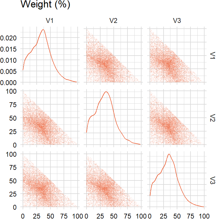

Approach 2(a): uniform sample from the simplex (http://mathoverflow.net/a/76258) and then normalize

If \(u\sim U(0,1)\) then \(-\ln(u)\) is an \(\text{Exp}(1)\) distribution

This is also known as generating a random vector from the symmetric Dirichlet distribution.

rand_weights2a <- function(n_sim, n_assets, lmbda) {
    
    # inverse transform sampling: https://en.wikipedia.org/wiki/Inverse_transform_sampling
    rand_exp <- matrix(-log(1 - runif(n_sim * n_assets)) / lmbda, nrow = n_sim, ncol = n_assets)
    result <- rand_exp / rowSums(rand_exp)
    
    return(result)
    
}

lmbda <- 1

approach2a <- rand_weights2a(n_sim, n_assets, lmbda)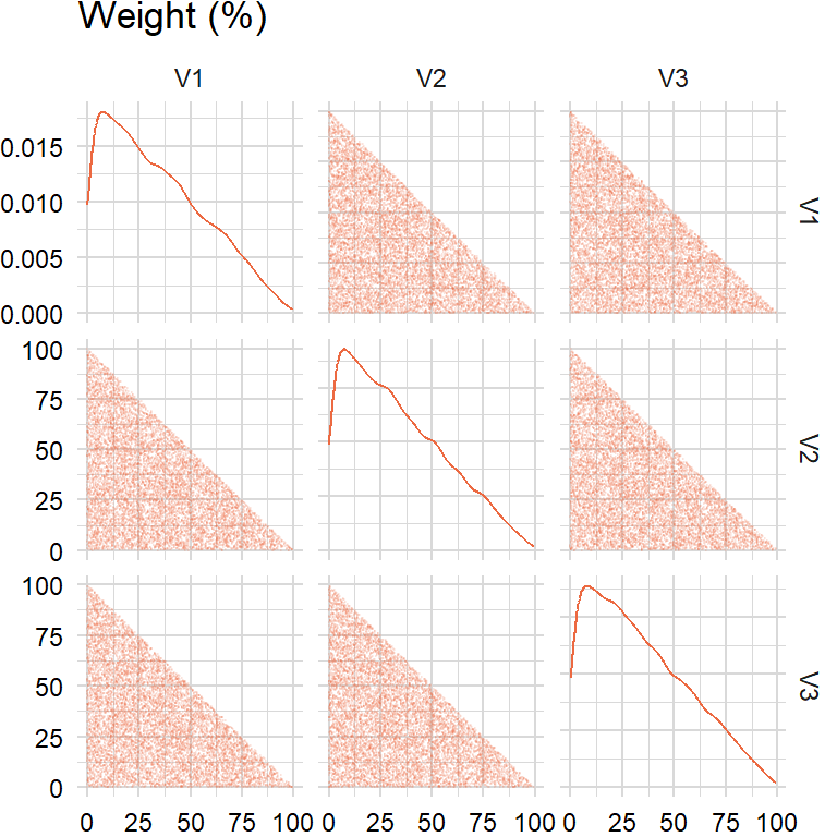

Approach 2(b): directly generate \(\text{Exp}(1)\) and then normalize

rand_weights2b <- function(n_sim, n_assets) {
    
    rand_exp <- matrix(rexp(n_sim * n_assets), nrow = n_sim, ncol = n_assets)
    result <- rand_exp / rowSums(rand_exp)
    
    return(result)
    
}

approach2b <- rand_weights2b(n_sim, n_assets)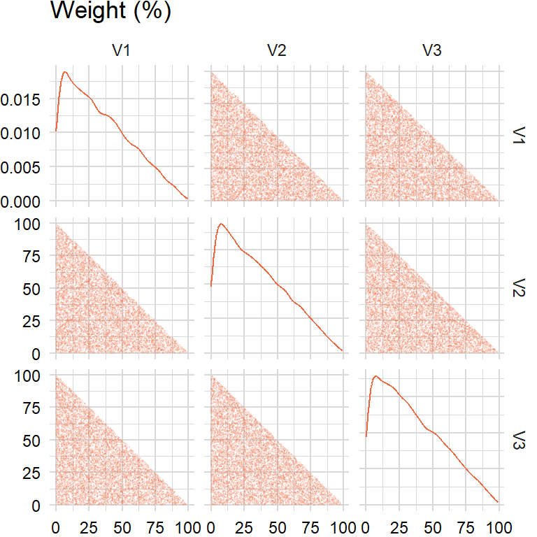

Random turnover

How to generate random weights between lower bound \(a\) and upper bound \(b\) that sum to zero?

Approach 1: tempting to multiply random weights by \(M\) and then subtract by \(\frac{M}{N}\) but the distribution is not between \(a\) and \(b\)
Approach 2: instead, use an iterative approach for random turnover:
1. Generate \(N-1\) uniformly distributed weights between \(a\) and \(b\)
2. For \(u_{N}\) compute sum of values and subtract from \(M\)
3. If \(u_{N}\) is between \(a\) and \(b\), then keep; otherwise, discard

Then add random turnover to previous period’s random weights.

rand_turnover1 <- function(n_sim, n_assets, lower, upper, target) {
    
    rng <- upper - lower
    
    result <- rand_weights2b(n_sim, n_assets) * rng
    result <- result - rng / n_assets
    
    return(result)
    
}

lower <- -0.05
upper <- 0.05
target <- 0

approach1 <- rand_turnover1(n_sim, n_assets, lower, upper, target)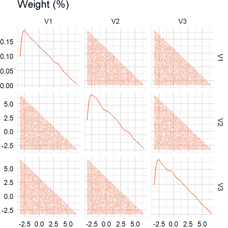

rand_iterative <- function(n_assets, lower, upper, target) {
    
    result <- runif(n_assets - 1, min = lower, max = upper)
    temp <- target - sum(result)
    
    while (!((temp <= upper) && (temp >= lower))) {
        
        result <- runif(n_assets - 1, min = lower, max = upper)
        temp <- target - sum(result)
        
    }
    
    result <- append(result, temp)
    
    return(result)
    
}

rand_turnover2 <- function(n_sim, n_assets, lower, upper, target) {
  
    result_ls <- list()
    
    for (i in 1:n_sim) {
        
        result_sim <- rand_iterative(n_assets, lower, upper, target)
        result_ls <- append(result_ls, list(result_sim))
        
    }
    
    result <- do.call(rbind, result_ls)
    
    return(result)
    
}

approach2 <- rand_turnover2(n_sim, n_assets, lower, upper, target)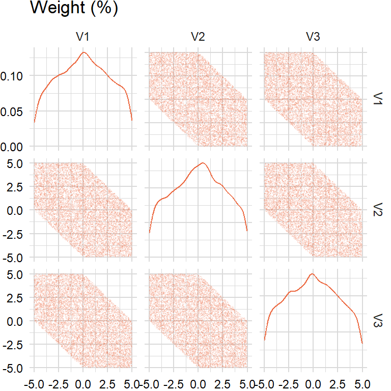

Mean-variance

library(CVXR)

geometric_mean <- function(x, scale) {
    
    result <- prod(1 + x) ^ (scale / length(x)) - 1
    
    return(result)
    
}

tickers <- "BAICX" # fund inception date is "2011-11-28"

returns_x_xts <- na.omit(returns_xts)[ , factors] # extended history
mu <- apply(returns_x_xts, 2, geometric_mean, scale = scale[["periods"]])
sigma <- cov(overlap_x_xts) * scale[["periods"]] * scale[["overlap"]]

Maximize means

\[ \begin{aligned} \begin{array}{rrcl} \displaystyle\min&-\mathbf{w}^{T}\mu\\ \textrm{s.t.}&\mathbf{w}^{T}e&=&1\\ &\mathbf{w}^T\Sigma\mathbf{w}&\leq&\sigma^{2}\\ \end{array} \end{aligned} \]

To incorporate these conditions into one equation, introduce new variables \(\lambda_{i}\) that are the Lagrange multipliers and define a new function \(\mathcal{L}\) as follows:

\[ \begin{aligned} \mathcal{L}(\mathbf{w},\lambda)&=-\mathbf{w}^{T}\mu-\lambda_{1}(\mathbf{w}^{T}e-1) \end{aligned} \]

Then, to minimize this function, take derivatives with respect to \(w\) and Lagrange multipliers \(\lambda_{i}\):

\[ \begin{aligned} \frac{\partial\mathcal{L}(\mathbf{w},\lambda)}{\partial w}&=-\mu-\lambda_{1}e=0\\ \frac{\partial\mathcal{L}(\mathbf{w},\lambda)}{\partial \lambda_{1}}&=\mathbf{w}e^T-1=0 \end{aligned} \]

Simplify the equations above in matrix form and solve for the Lagrange multipliers \(\lambda_{i}\):

\[ \begin{aligned} \begin{bmatrix} -\mu & e \\ e^{T} & 0 \end{bmatrix} \begin{bmatrix} \mathbf{w} \\ -\lambda_{1} \end{bmatrix} &= \begin{bmatrix} 0 \\ 1 \end{bmatrix} \\ \begin{bmatrix} \mathbf{w} \\ -\lambda_{1} \end{bmatrix} &= \begin{bmatrix} -\mu & e \\ e^{T} & 0 \end{bmatrix}^{-1} \begin{bmatrix} 0 \\ 1 \end{bmatrix} \end{aligned} \]

max_mean_optim <- function(mu, sigma, target) {
    
    params <- Variable(length(mu))
    
    obj <- Maximize(t(params) %*% mu)
    
    cons <- list(sum(params) == 1, params >= 0,
                 quad_form(params, sigma) <= target ^ 2)
    
    prob <- Problem(obj, cons)
    
    result <- solve(prob)$getValue(params)
    
    return(result)

}

target <- 0.06

params1 <- t(max_mean_optim(mu, sigma, target))
params1

          [,1]      [,2]         [,3]         [,4]
[1,] 0.4961023 0.5038977 7.919319e-09 4.929859e-09

params1 %*% mu

          [,1]
[1,] 0.0472976

sqrt(params1 %*% sigma %*% t(params1))

     [,1]
[1,] 0.06

# # install.packages("devtools")
# devtools::install_github("jasonjfoster/rolloptim") # roll (>= 1.1.7)
# library(rolloptim)
# 
# mu <- roll_mean(returns_x_xts, 5)
# sigma <- roll_cov(returns_x_xts, width = 5)
# 
# xx <- roll_crossprod(returns_x_xts, returns_x_xts, 5)
# xy <- roll_crossprod(returns_x_xts, returns_y_xts, 5)
# 
# roll_max_mean(mu)

Minimize variance

\[ \begin{aligned} \begin{array}{rrcl} \displaystyle\min&\frac{1}{2}\mathbf{w}^T\Sigma\mathbf{w}\\ \textrm{s.t.}&\mathbf{w}^{T}e&=&1\\ &\mu^{T}\mathbf{w}&\geq&M\\ \end{array} \end{aligned} \]

To incorporate these conditions into one equation, introduce new variables \(\lambda_{i}\) that are the Lagrange multipliers and define a new function \(\mathcal{L}\) as follows:

\[ \begin{aligned} \mathcal{L}(\mathbf{w},\lambda)&=\frac{1}{2}\mathbf{w}^{T}\Sigma\mathbf{w}-\lambda_{1}(\mathbf{w}^{T}e-1) \end{aligned} \]

Then, to minimize this function, take derivatives with respect to \(w\) and Lagrange multipliers \(\lambda_{i}\):

\[ \begin{aligned} \frac{\partial\mathcal{L}(\mathbf{w},\lambda)}{\partial w}&=\mathbf{w}\Sigma-\lambda_{1}e=0\\ \frac{\partial\mathcal{L}(\mathbf{w},\lambda)}{\partial \lambda_{1}}&=\mathbf{w}e^T-1=0 \end{aligned} \]

Simplify the equations above in matrix form and solve for the Lagrange multipliers \(\lambda_{i}\):

\[ \begin{aligned} \begin{bmatrix} \Sigma & e \\ e^{T} & 0 \end{bmatrix} \begin{bmatrix} \mathbf{w} \\ -\lambda_{1} \end{bmatrix} &= \begin{bmatrix} 0 \\ 1 \end{bmatrix} \\ \begin{bmatrix} \mathbf{w} \\ -\lambda_{1} \end{bmatrix} &= \begin{bmatrix} \Sigma & e \\ e^{T} & 0 \end{bmatrix}^{-1} \begin{bmatrix} 0 \\ 1 \end{bmatrix} \end{aligned} \]

min_var_optim <- function(mu, sigma, target) {
    
    params <- Variable(length(mu))
    
    obj <- Minimize(quad_form(params, sigma))
    
    cons <- list(sum(params) == 1, params >= 0,
                 sum(mu * params) >= target)
    
    prob <- Problem(obj, cons)
    
    result <- solve(prob)$getValue(params)
    
    return(result)

}

target <- 0.03

params2 <- t(min_var_optim(mu, sigma, target))
params2

        [,1]      [,2]      [,3]         [,4]
[1,] 0.29584 0.4463629 0.2577972 1.877369e-21

params2 %*% mu

     [,1]
[1,] 0.03

sqrt(params2 %*% sigma %*% t(params2))

          [,1]
[1,] 0.0372178

# roll_min_var(sigma)

Maximize utility

\[ \begin{aligned} \begin{array}{rrcl} \displaystyle\min&\frac{1}{2}\delta(\mathbf{w}^{T}\Sigma\mathbf{w})-\mu^{T}\mathbf{w}\\ \textrm{s.t.}&\mathbf{w}^{T}e&=&1\\ \end{array} \end{aligned} \]

To incorporate these conditions into one equation, introduce new variables \(\lambda_{i}\) that are the Lagrange multipliers and define a new function \(\mathcal{L}\) as follows:

\[ \begin{aligned} \mathcal{L}(\mathbf{w},\lambda)&=\frac{1}{2}\mathbf{w}^{T}\Sigma\mathbf{w}-\mu^{T}\mathbf{w}-\lambda_{1}(\mathbf{w}^{T}e-1) \end{aligned} \]

Then, to minimize this function, take derivatives with respect to \(w\) and Lagrange multipliers \(\lambda_{i}\):

\[ \begin{aligned} \frac{\partial\mathcal{L}(\mathbf{w},\lambda)}{\partial w}&=\mathbf{w}\Sigma-\mu^{T}-\lambda_{1}e=0\\ \frac{\partial\mathcal{L}(\mathbf{w},\lambda)}{\partial \lambda_{1}}&=\mathbf{w}e^T-1=0 \end{aligned} \]

Simplify the equations above in matrix form and solve for the Lagrange multipliers \(\lambda_{i}\):

\[ \begin{aligned} \begin{bmatrix} \Sigma & e \\ e^{T} & 0 \end{bmatrix} \begin{bmatrix} \mathbf{w} \\ -\lambda_{1} \end{bmatrix} &= \begin{bmatrix} \mu^{T} \\ 1 \end{bmatrix} \\ \begin{bmatrix} \mathbf{w} \\ -\lambda_{1} \end{bmatrix} &= \begin{bmatrix} \Sigma & e \\ e^{T} & 0 \end{bmatrix}^{-1} \begin{bmatrix} \mu^{T} \\ 1 \end{bmatrix} \end{aligned} \]

max_utility_optim <- function(mu, sigma, target) {
    
    params <- Variable(length(mu))
    
    obj <- Minimize(0.5 * target * quad_form(params, sigma) - t(mu) %*% params)
    
    cons <- list(sum(params) == 1, params >= 0)
    
    prob <- Problem(obj, cons)
        
    result <- solve(prob)$getValue(params)
    
    return(result)

}

ir <- 0.5
target <- ir / 0.06 # ir / std (see Black-Litterman)

params3 <- t(max_utility_optim(mu, sigma, target))
params3

          [,1]      [,2]         [,3]         [,4]
[1,] 0.5584661 0.4415339 9.327449e-23 4.233534e-23

params3 %*% mu

           [,1]
[1,] 0.05158278

sqrt(params3 %*% sigma %*% t(params3))

          [,1]
[1,] 0.0672845

# roll_max_utility(mu, sigma)

Minimize residual sum of squares

\[ \begin{aligned} \begin{array}{rrcl} \displaystyle\min&\frac{1}{2}\delta(\mathbf{w}^{T}X^{T}X\mathbf{w})-X^{T}y\mathbf{w}\\ \textrm{s.t.}&\mathbf{w}^{T}e&=&1\\ \end{array} \end{aligned} \]

To incorporate these conditions into one equation, introduce new variables \(\lambda_{i}\) that are the Lagrange multipliers and define a new function \(\mathcal{L}\) as follows:

\[ \begin{aligned} \mathcal{L}(\mathbf{w},\lambda)&=\frac{1}{2}\mathbf{w}^{T}X^{T}X\mathbf{w}-X^{T}y\mathbf{w}-\lambda_{1}(\mathbf{w}^{T}e-1) \end{aligned} \]

Then, to minimize this function, take derivatives with respect to \(w\) and Lagrange multipliers \(\lambda_{i}\):

\[ \begin{aligned} \frac{\partial\mathcal{L}(\mathbf{w},\lambda)}{\partial w}&=\mathbf{w}X^{T}X-X^{T}y-\lambda_{1}e=0\\ \frac{\partial\mathcal{L}(\mathbf{w},\lambda)}{\partial \lambda_{1}}&=\mathbf{w}e^T-1=0 \end{aligned} \]

Simplify the equations above in matrix form and solve for the Lagrange multipliers \(\lambda_{i}\):

\[ \begin{aligned} \begin{bmatrix} X^{T}X & e \\ e^{T} & 0 \end{bmatrix} \begin{bmatrix} \mathbf{w} \\ -\lambda_{1} \end{bmatrix} &= \begin{bmatrix} X^{T}y \\ 1 \end{bmatrix} \\ \begin{bmatrix} \mathbf{w} \\ -\lambda_{1} \end{bmatrix} &= \begin{bmatrix} X^{T}X & e \\ e^{T} & 0 \end{bmatrix}^{-1} \begin{bmatrix} X^{T}y \\ 1 \end{bmatrix} \end{aligned} \]

https://scaron.info/blog/conversion-from-least-squares-to-quadratic-programming.html

min_rss_optim1 <- function(mu, sigma) {
    
    params <- Variable(length(mu))
    
    obj <- Minimize(0.5 * quad_form(params, sigma) - t(mu) %*% params)
    
    cons <- list(sum(params) == 1, params >= 0)
    
    prob <- Problem(obj, cons)
        
    result <- solve(prob)$getValue(params)
    
    return(result)

}

params4 <- t(min_rss_optim1(crossprod(overlap_x_xts, overlap_y_xts), crossprod(overlap_x_xts)))
params4

         [,1]         [,2]     [,3]         [,4]
[1,] 0.374955 7.191451e-23 0.625045 2.959672e-23

params4 %*% mu

           [,1]
[1,] 0.03039745

sqrt(params4 %*% sigma %*% t(params4))

           [,1]
[1,] 0.05050206

# roll_min_rss(xx, xy)

min_rss_optim2 <- function(x, y) {
    
    params <- Variable(ncol(x))
    
    obj <- Minimize(sum_squares(y - x %*% params))
    
    cons <- list(sum(params) == 1, params >= 0)
    
    prob <- Problem(obj, cons)
        
    result <- solve(prob)$getValue(params)
    
    return(result)

}

params5 <- t(min_rss_optim2(coredata(overlap_x_xts), coredata(overlap_y_xts)))
params5

         [,1]          [,2]     [,3]          [,4]
[1,] 0.374955 -1.364843e-20 0.625045 -8.927092e-21

params5 %*% mu

           [,1]
[1,] 0.03039745

sqrt(params5 %*% sigma %*% t(params5))

           [,1]
[1,] 0.05050206

round(data.frame("max_pnl" = t(params1) * 100,
                 "min_risk" = t(params2) * 100,
                 "max_utility" = t(params3) * 100,
                 "min_rss1" = t(params4) * 100,
                 "min_rss2" = t(params5) * 100), 2)

  max_pnl min_risk max_utility min_rss1 min_rss2
1   49.61    29.58       55.85     37.5     37.5
2   50.39    44.64       44.15      0.0      0.0
3    0.00    25.78        0.00     62.5     62.5
4    0.00     0.00        0.00      0.0      0.0