Optimization

factors_r = ["SP500", "DTWEXAFEGS"] # "SP500" does not contain dividends; note: "DTWEXM" discontinued as of Jan 2020
factors_d = ["DGS10", "BAMLH0A0HYM2"]

Random weights

Need to generate uniformly distributed weights \(\mathbf{w}=(w_{1},w_{2},\ldots,w_{N})\) such that \(\sum_{j=1}^{N}w_{i}=1\) and \(w_{i}\geq0\):

• Approach 1: tempting to use \(w_{i}=\frac{u_{i}}{\sum_{j=1}^{N}u_{i}}\) where \(u_{i}\sim U(0,1)\) but the distribution of \(\mathbf{w}\) is not uniform

• Approach 2: instead, generate \(\text{Exp}(1)\) and then normalize

Can also scale random weights by \(M\), e.g. if sum of weights must be 10% then multiply weights by 10%.

def rand_weights1(n_sim, n_assets):  
    
    rand_exp = np.matrix(np.random.uniform(size = (n_sim, n_assets)))
    rand_exp_sum = np.sum(rand_exp, axis = 1)
    
    result = rand_exp / rand_exp_sum
    
    return result

n_assets = 3
n_sim = 10000

approach1 = rand_weights1(n_sim, n_assets)

Approach 2(a): uniform sample from the simplex (http://mathoverflow.net/a/76258) and then normalize

• If \(u\sim U(0,1)\) then \(-\ln(u)\) is an \(\text{Exp}(1)\) distribution

This is also known as generating a random vector from the symmetric Dirichlet distribution.

def rand_weights2a(n_sim, n_assets, lmbda):   
    
    # inverse transform sampling: https://en.wikipedia.org/wiki/Inverse_transform_sampling
    rand_exp = np.matrix(-np.log(1 - np.random.uniform(size = (n_sim, n_assets))) / lmbda)
    rand_exp_sum = np.sum(rand_exp, axis = 1)
    
    result = rand_exp / rand_exp_sum
    
    return result

lmbda = 1

approach2a = rand_weights2a(n_sim, n_assets, lmbda)

Approach 2(b): directly generate \(\text{Exp}(1)\) and then normalize

def rand_weights2b(n_sim, n_assets):
    
    rand_exp = np.matrix(np.random.exponential(size = (n_sim, n_assets)))
    rand_exp_sum = np.sum(rand_exp, axis = 1)
    
    result = rand_exp / rand_exp_sum
    
    return result

approach2b = rand_weights2b(n_sim, n_assets)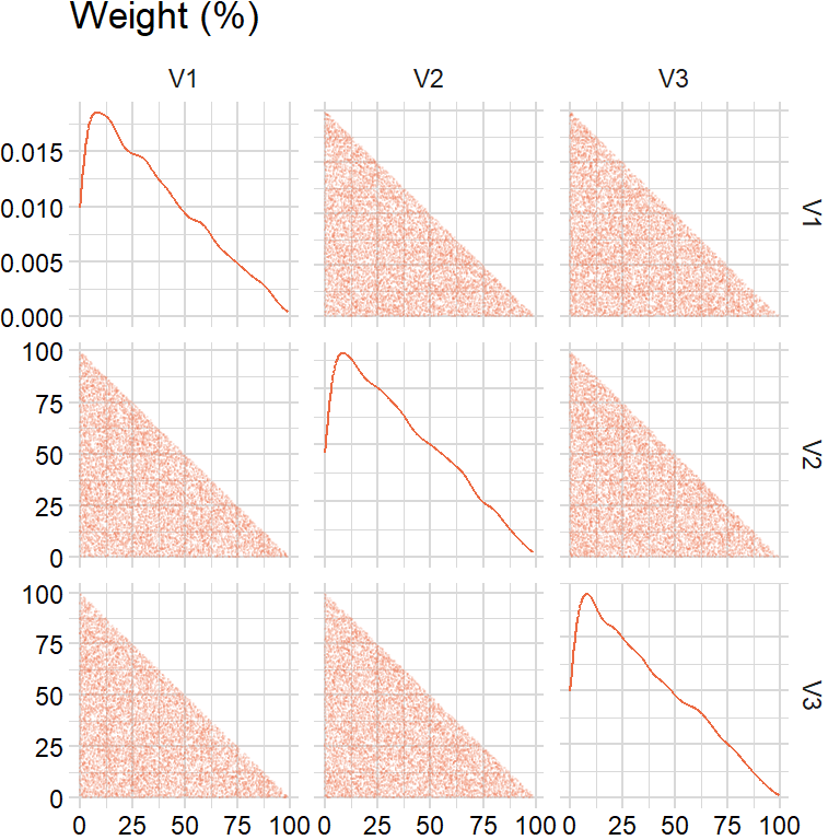

Random turnover

How to generate random weights between lower bound \(a\) and upper bound \(b\) that sum to zero?

• Approach 1: tempting to multiply random weights by \(M\) and then subtract by \(\frac{M}{N}\) but the distribution is not between \(a\) and \(b\)

• Approach 2: instead, use an iterative approach for random turnover:

  1. Generate \(N-1\) uniformly distributed weights between \(a\) and \(b\)
  2. For \(u_{N}\) compute sum of values and subtract from \(M\)
  3. If \(u_{N}\) is between \(a\) and \(b\), then keep; otherwise, discard

Then add random turnover to previous period’s random weights.

def rand_turnover1(n_sim, n_assets, lower, upper, target):
    
    rng = upper - lower
    
    result = rand_weights2b(n_sim, n_assets) * rng
    result = result - rng / n_assets
    
    return result

lower = -0.05
upper = 0.05
target = 0

approach1 = rand_turnover1(n_sim, n_assets, lower, upper, target)

def rand_iterative(n_assets, lower, upper, target):
    
    result = np.random.uniform(low = lower, high = upper, size = n_assets - 1)
    temp = target - sum(result)
    
    while not ((temp <= upper) and (temp >= lower)):
        result = np.random.uniform(low = lower, high = upper, size = n_assets - 1)
        temp = target - sum(result)
        
    result = np.append(result, temp)
    
    return result

def rand_turnover2(n_sim, n_assets, lower, upper, target):
  
    result_ls = []
    
    for i in range(n_sim):
      
      result_sim = rand_iterative(n_assets, lower, upper, target)
      result_ls.append(result_sim)
      
    result = pd.DataFrame(result_ls)
    
    return result

approach2 = rand_turnover2(n_sim, n_assets, lower, upper, target)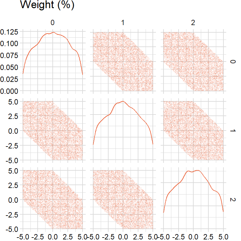

Mean-variance

import cvxpy as cp

def geometric_mean(x, scale):
    
    result = np.prod(1 + x) ** (scale/ len(x)) - 1
    
    return result

• https://www.adrian.idv.hk/2021-06-22-kkt/
• https://or.stackexchange.com/a/3738
• https://bookdown.org/compfinezbook/introFinRbook/Portfolio-Theory-with-Matrix-Algebra.html#algorithm-for-computing-efficient-frontier
• https://palomar.home.ece.ust.hk/MAFS6010R_lectures/slides_robust_portfolio.html

tickers = ["BAICX"] # fund inception date is "2011-11-28"

returns_x_df = returns_df.dropna()[factors]
mu = returns_x_df.apply(geometric_mean, axis = 0, scale = scale["periods"])
sigma = np.cov(overlap_x_df.T, ddof = 1) * scale["periods"] * scale["overlap"]

Maximize mean

\[ \begin{aligned} \begin{array}{rrcl} \displaystyle\min&-\mathbf{w}^{T}\mu\\ \textrm{s.t.}&\mathbf{w}^{T}e&=&1\\ &\mathbf{w}^T\Sigma\mathbf{w}&\leq&\sigma^{2}\\ \end{array} \end{aligned} \]

To incorporate these conditions into one equation, introduce new variables \(\lambda_{i}\) that are the Lagrange multipliers and define a new function \(\mathcal{L}\) as follows:

\[ \begin{aligned} \mathcal{L}(\mathbf{w},\lambda)&=-\mathbf{w}^{T}\mu-\lambda_{1}(\mathbf{w}^{T}e-1) \end{aligned} \]

Then, to minimize this function, take derivatives with respect to \(w\) and Lagrange multipliers \(\lambda_{i}\):

\[ \begin{aligned} \frac{\partial\mathcal{L}(\mathbf{w},\lambda)}{\partial w}&=-\mu-\lambda_{1}e=0\\ \frac{\partial\mathcal{L}(\mathbf{w},\lambda)}{\partial \lambda_{1}}&=\mathbf{w}e^T-1=0 \end{aligned} \]

Simplify the equations above in matrix form and solve for the Lagrange multipliers \(\lambda_{i}\):

\[ \begin{aligned} \begin{bmatrix} -\mu & e \\ e^{T} & 0 \end{bmatrix} \begin{bmatrix} \mathbf{w} \\ -\lambda_{1} \end{bmatrix} &= \begin{bmatrix} 0 \\ 1 \end{bmatrix} \\ \begin{bmatrix} \mathbf{w} \\ -\lambda_{1} \end{bmatrix} &= \begin{bmatrix} -\mu & e \\ e^{T} & 0 \end{bmatrix}^{-1} \begin{bmatrix} 0 \\ 1 \end{bmatrix} \end{aligned} \]

def max_mean_optim(mu, sigma, target):
    
    params = cp.Variable(len(mu))
    
    obj = cp.Maximize(params.T @ mu)
    
    cons = [cp.sum(params) == 1, params >= 0,
            cp.quad_form(params, sigma) <= target ** 2]
    
    prob = cp.Problem(obj, cons)
    
    prob.solve()
    
    return params.value

target = 0.06

params1 = max_mean_optim(mu, sigma, target)
params1

array([4.31211361e-01, 2.11082389e-01, 2.44018500e-06, 3.57703809e-01])

np.dot(mu, params1)

np.float64(0.04387993526045541)

np.sqrt(np.dot(params1, np.dot(sigma, params1)))

np.float64(0.059999998673826355)

Minimize variance

\[ \begin{aligned} \begin{array}{rrcl} \displaystyle\min&\frac{1}{2}\mathbf{w}^T\Sigma\mathbf{w}\\ \textrm{s.t.}&\mathbf{w}^{T}e&=&1\\ &\mu^{T}\mathbf{w}&\geq&M\\ \end{array} \end{aligned} \]

To incorporate these conditions into one equation, introduce new variables \(\lambda_{i}\) that are the Lagrange multipliers and define a new function \(\mathcal{L}\) as follows:

\[ \begin{aligned} \mathcal{L}(\mathbf{w},\lambda)&=\frac{1}{2}\mathbf{w}^{T}\Sigma\mathbf{w}-\lambda_{1}(\mathbf{w}^{T}e-1) \end{aligned} \]

Then, to minimize this function, take derivatives with respect to \(w\) and Lagrange multipliers \(\lambda_{i}\):

\[ \begin{aligned} \frac{\partial\mathcal{L}(\mathbf{w},\lambda)}{\partial w}&=\mathbf{w}\Sigma-\lambda_{1}e=0\\ \frac{\partial\mathcal{L}(\mathbf{w},\lambda)}{\partial \lambda_{1}}&=\mathbf{w}e^T-1=0 \end{aligned} \]

Simplify the equations above in matrix form and solve for the Lagrange multipliers \(\lambda_{i}\):

\[ \begin{aligned} \begin{bmatrix} \Sigma & e \\ e^{T} & 0 \end{bmatrix} \begin{bmatrix} \mathbf{w} \\ -\lambda_{1} \end{bmatrix} &= \begin{bmatrix} 0 \\ 1 \end{bmatrix} \\ \begin{bmatrix} \mathbf{w} \\ -\lambda_{1} \end{bmatrix} &= \begin{bmatrix} \Sigma & e \\ e^{T} & 0 \end{bmatrix}^{-1} \begin{bmatrix} 0 \\ 1 \end{bmatrix} \end{aligned} \]

def min_var_optim(mu, sigma, target):
    
    params = cp.Variable(len(mu))
    
    obj = cp.Minimize(cp.quad_form(params, sigma))
    
    cons = [cp.sum(params) == 1, params >= 0,
            params.T @ mu >= target]
    
    prob = cp.Problem(obj, cons)
    
    prob.solve()
    
    return params.value

target = 0.03

params2 = min_var_optim(mu, sigma, target)
params2

array([ 2.83586236e-01,  1.48145971e-01, -2.59839572e-20,  5.68267794e-01])

np.dot(mu, params2)

np.float64(0.029999999999999992)

np.sqrt(np.dot(params2, np.dot(sigma, params2))) 

np.float64(0.04156129001157303)

Maximize utility

\[ \begin{aligned} \begin{array}{rrcl} \displaystyle\min&\frac{1}{2}\delta(\mathbf{w}^{T}\Sigma\mathbf{w})-\mu^{T}\mathbf{w}\\ \textrm{s.t.}&\mathbf{w}^{T}e&=&1\\ \end{array} \end{aligned} \]

To incorporate these conditions into one equation, introduce new variables \(\lambda_{i}\) that are the Lagrange multipliers and define a new function \(\mathcal{L}\) as follows:

\[ \begin{aligned} \mathcal{L}(\mathbf{w},\lambda)&=\frac{1}{2}\mathbf{w}^{T}\Sigma\mathbf{w}-\mu^{T}\mathbf{w}-\lambda_{1}(\mathbf{w}^{T}e-1) \end{aligned} \]

Then, to minimize this function, take derivatives with respect to \(w\) and Lagrange multipliers \(\lambda_{i}\):

\[ \begin{aligned} \frac{\partial\mathcal{L}(\mathbf{w},\lambda)}{\partial w}&=\mathbf{w}\Sigma-\mu^{T}-\lambda_{1}e=0\\ \frac{\partial\mathcal{L}(\mathbf{w},\lambda)}{\partial \lambda_{1}}&=\mathbf{w}e^T-1=0 \end{aligned} \]

Simplify the equations above in matrix form and solve for the Lagrange multipliers \(\lambda_{i}\):

\[ \begin{aligned} \begin{bmatrix} \Sigma & e \\ e^{T} & 0 \end{bmatrix} \begin{bmatrix} \mathbf{w} \\ -\lambda_{1} \end{bmatrix} &= \begin{bmatrix} \mu^{T} \\ 1 \end{bmatrix} \\ \begin{bmatrix} \mathbf{w} \\ -\lambda_{1} \end{bmatrix} &= \begin{bmatrix} \Sigma & e \\ e^{T} & 0 \end{bmatrix}^{-1} \begin{bmatrix} \mu^{T} \\ 1 \end{bmatrix} \end{aligned} \]

def max_utility_optim(mu, sigma, target):
    
    params = cp.Variable(len(mu))
    
    obj = cp.Minimize(0.5 * target * cp.quad_form(params, sigma) - params.T @ mu)
    
    cons = [cp.sum(params) == 1, params >= 0]
    
    prob = cp.Problem(obj, cons)
    
    prob.solve()
    
    return params.value

ir = 0.5
target = ir / 0.06 # ir / std (see Black-Litterman)

params3 = max_utility_optim(mu, sigma, target)
params3

array([6.65831063e-01, 3.11106711e-01, 1.73830812e-23, 2.30622261e-02])

np.dot(mu, params3)

np.float64(0.06593926158420194)

np.sqrt(np.matmul(np.transpose(params3), np.matmul(sigma, params3)))

np.float64(0.08951308848063624)

Minimize residual sum of squares

\[ \begin{aligned} \begin{array}{rrcl} \displaystyle\min&\frac{1}{2}\delta(\mathbf{w}^{T}X^{T}X\mathbf{w})-X^{T}y\mathbf{w}\\ \textrm{s.t.}&\mathbf{w}^{T}e&=&1\\ \end{array} \end{aligned} \]

To incorporate these conditions into one equation, introduce new variables \(\lambda_{i}\) that are the Lagrange multipliers and define a new function \(\mathcal{L}\) as follows:

\[ \begin{aligned} \mathcal{L}(\mathbf{w},\lambda)&=\frac{1}{2}\mathbf{w}^{T}X^{T}X\mathbf{w}-X^{T}y\mathbf{w}-\lambda_{1}(\mathbf{w}^{T}e-1) \end{aligned} \]

Then, to minimize this function, take derivatives with respect to \(w\) and Lagrange multipliers \(\lambda_{i}\):

\[ \begin{aligned} \frac{\partial\mathcal{L}(\mathbf{w},\lambda)}{\partial w}&=\mathbf{w}X^{T}X-X^{T}y-\lambda_{1}e=0\\ \frac{\partial\mathcal{L}(\mathbf{w},\lambda)}{\partial \lambda_{1}}&=\mathbf{w}e^T-1=0 \end{aligned} \]

Simplify the equations above in matrix form and solve for the Lagrange multipliers \(\lambda_{i}\):

\[ \begin{aligned} \begin{bmatrix} X^{T}X & e \\ e^{T} & 0 \end{bmatrix} \begin{bmatrix} \mathbf{w} \\ -\lambda_{1} \end{bmatrix} &= \begin{bmatrix} X^{T}y \\ 1 \end{bmatrix} \\ \begin{bmatrix} \mathbf{w} \\ -\lambda_{1} \end{bmatrix} &= \begin{bmatrix} X^{T}X & e \\ e^{T} & 0 \end{bmatrix}^{-1} \begin{bmatrix} X^{T}y \\ 1 \end{bmatrix} \end{aligned} \]

• https://scaron.info/blog/conversion-from-least-squares-to-quadratic-programming.html

def min_rss_optim1(mu, sigma):
    
    params = cp.Variable(len(mu))
    
    obj = cp.Minimize(0.5 * cp.quad_form(params, sigma) - params.T @ mu)
    
    cons = [cp.sum(params) == 1, params >= 0]
    
    prob = cp.Problem(obj, cons)
    
    prob.solve()
    
    return params.value

params4 = min_rss_optim1(np.dot(overlap_x_df.T.values, overlap_y_df.values),
                         np.dot(overlap_x_df.T.values, overlap_x_df.values))
params4

array([2.79223870e-01, 8.10663395e-24, 7.20776130e-01, 1.15062333e-23])

np.dot(mu, params4)

np.float64(0.026104599832123966)

np.sqrt(np.matmul(np.transpose(params4), np.matmul(sigma, params4)))

np.float64(0.03913103713942823)

def min_rss_optim2(x, y):
    
    params = cp.Variable(x.shape[1])
    
    obj = cp.Minimize(cp.sum_squares(y - x @ params))
    
    cons = [cp.sum(params) == 1, params >= 0]
    
    prob = cp.Problem(obj, cons)
    
    prob.solve()
    
    return params.value

params5 = min_rss_optim2(overlap_x_df.values, overlap_y_df.iloc[:, 0].values)
params5

array([ 2.79223870e-01, -1.61222438e-20,  7.20776130e-01, -1.43092675e-20])

np.dot(mu, params5)

np.float64(0.02610459983212409)

np.sqrt(np.matmul(np.transpose(params5), np.matmul(sigma, params5)))

np.float64(0.0391310371394284)

pd.DataFrame({
  "max_pnl": params1 * 100,
  "min_risk": params2 * 100,
  "max_utility": params3 * 100,
  "min_rss1": params4 * 100,
  "min_rss2": params5 * 100
}).round(2)

   max_pnl  min_risk  max_utility  min_rss1  min_rss2
0    43.12     28.36        66.58     27.92     27.92
1    21.11     14.81        31.11      0.00     -0.00
2     0.00     -0.00         0.00     72.08     72.08
3    35.77     56.83         2.31      0.00     -0.00